MS SQL SMS export large data to Excel without breaking format

If you often work on MS SQL, surely sometimes you want to export large data (result a query) to Excel file. After querying on MS SQL SMS (Microsoft SQL Server Management Studio), you can use right click on the cell top left then select "Copy with Headers" and copy to Excel file or "Save Result As" and save to a CSV file.

However 2 these functions have their problems. "Copy with Headers" cannot copy large data.  "Save Result As" often breaks CSV format if your data contains some special characters.

Fortunately, there is another function for exporting large data without breaking its format. Right click on your database and choose Tasks >> Export Data...

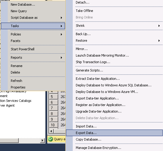
For Data Source, choose SQL Server Native >> select Server name >> select your Database, see the following for example:

Next, select Destination as Microsoft Excel & specify Excel file path.

Next, select Write a query to specify the data to transfer.

In next step, paste your query into or select a file containing your query. In the step Review Data Type Mapping, let review again columns have been converted data (Source Type vs. Destination Type). If you want to fix, click Back to select again Destination Type for converting.

If they are ok, click Next then Finish (don't worry for warning signs). Waiting a moment and you will have your Excel file with correct format you wanted.

Yeah! This is a small tip for you, hope it is useful. Share it to your friend for helping him or her out 😍. Any comment is welcome!

Happy Halloween!

Excel: How to remove empty area and make worksheets nicer for printing

Almost time when using Excel, I need to print its worksheets as result of my work.

But sometimes, I use File >> Print Preview to see what the document will look like if I print it, I often see that the document gets many extra blank pages or the columns broken into new pages. If I save the document as a .pdf file, the problem persists in the .pdf file. It's worse.

However, Excel has Page Layout functions groups to help us make worksheets nicer. Below are 2 functions I often use:

• Page Layout >> Page Setup >> Print Area >> Set Print Area: select area which you want to print and use this function
• Page Layout >> Scale to fit >> Width: should be set to 1 page, it will help to avoid broken columns.

There are a lot of functions there which you can try and see until you feel it's good.
Yes, let remember to use Print Preview function to check again before printing any document.
Any comment is welcome.

Bye, nice day!
Hung

Excel: Merge cells in rows having same values

All most people like me and you often use Excel to process Data. Some times you get a Data with cells in rows having same values, and you want to merge them into 1 cell by each column. For example, you have a Data like the screenshot below:

And you want to achieve new Data as the following:

In which, SUM column will have new value = SUM of rows on AllOrHalf column which are belong to the merged cell.

In this article, I'll show you a solution using VBA to make this work. On the sheet, press Alt+F11 to open Visual Basic Editor (VBE). Right click on your workbook name in the Project-VBAProject pane (at the top left corner of the editor window) and select Insert >> Module from the context menu.

Copy below code to the window:

Option Explicit

Private Sub MergeCells()
    Application.ScreenUpdating = False
    Application.DisplayAlerts = False

    Dim rngMerge As Range, cell As Range
    Dim nrow As Integer: nrow = 0
    Dim continue As Boolean: continue = True
    Dim totalLeave As Double: totalLeave = 0
    Set rngMerge = Range("A2:A9") 'range to check
    

    For Each cell In rngMerge
        Do
            totalLeave = totalLeave + cell.Offset(nrow, 5).Value
            If cell.Offset(nrow, 0).Value = cell.Offset(nrow + 1, 0).Value _
              And cell.Offset(nrow, 1).Value = cell.Offset(nrow + 1, 1).Value _
              And cell.Offset(nrow, 2).Value = cell.Offset(nrow + 1, 2).Value _
              And cell.Offset(nrow, 3).Value = cell.Offset(nrow + 1, 3).Value _
              And IsEmpty(cell) = False Then
                nrow = nrow + 1 'check next row
                continue = True
            Else
                continue = False
            End If
        Loop Until continue = False
        If nrow > 0 Then
            Range(cell.Offset(0, 3), cell.Offset(nrow, 3)).Merge
            Range(cell.Offset(0, 2), cell.Offset(nrow, 2)).Merge
            Range(cell.Offset(0, 1), cell.Offset(nrow, 1)).Merge
            Range(cell, cell.Offset(nrow, 0)).Merge
            nrow = 0
        End If
        cell.Offset(0, 3).Value = totalLeave 'assign value to SUM column
        totalLeave = 0
    Next
    
    Application.DisplayAlerts = True
    Application.ScreenUpdating = True
End Sub

Then press F5 to run the code. After that, you can format merged cells and you will get the result.

That's it. Any comment is welcome.

Excel: Create Pie chart from single column

1. Add new column (e.g. Count) and fill it with 1
   
2. Select your data (both columns) and create a Pivot Table: On the Insert tab click on the PivotTable | Pivot Table (you can create it on the same worksheet or on a new sheet)
   
3. On the PivotTable Filed List drag Country to Row Labels and Count to Values
   
4. Now select the pivot table data and create your pie chart as usual.
   

P.S. I use the pivot table for I update the data on a regular basis, then I just replace the "Country" data and refresh the pivot table.